Finding the needle without searching the entire haystack

Image by Jakub Żerdzicki retrieved from Unsplash

Linear Optimization is one of the most powerful tools in Operations Research. However, when we add the realistic constraint that variables must be integer numbers (such as the number of trucks to charter, factories to open, or personnel to hire), the problem changes categories drastically.

Naive rounding of the continuous solution rarely works and often leads to infeasible solutions or solutions far from the true optimum. To solve this challenge without falling into a computationally impossible exhaustive search, the Branch and Bound algorithm stands out as one of the benchmarks.

A Brief Historical Context

The basic concept of the branch and bound procedure emerged in the early 1960s:

• 1960: Researchers Ailsa Land and Alison Harcourt (Doig) published the pioneering work (Land & Doig, 1960) that gave birth to the branch and bound methodology for solving discrete numerical problems.
• 1965: R. J. Dakin formulated a variation tailored to Integer Optimization (Dakin, 1965) based on partitioning the search space using constraints on fractional variables, leading to the hierarchical tree structure as we know it today.

Core Concepts

To understand branch and bound, let us imagine a smart “divide and conquer” process supported by three pillars (assuming a minimization problem):

1. Continuous Relaxation: This consists of solving the problem by temporarily dropping the integrality conditions on the variables. This allows us to apply fast algorithms (such as Simplex or Interior Point) and obtain a theoretical bound on the best possible value.

2. Branching: If the relaxed solution yields a non-integer value for a variable $x_k^*$ that should be an integer, we split the original problem into two mutually exclusive subproblems by adding new constraints: \(x_k \leqslant \lfloor x_k^* \rfloor\) and \(x_k \geqslant \lceil x_k^* \rceil\) which allow us to disregard a region where no integer solutions can exist.

3. Bounding: As we explore the tree of subproblems, we keep track of the bounds:

   • Lower Bound ($z_S$): The objective function value at the relaxed nodes.
   • Upper Bound ($z_I$): The objective value of the best integer solution known so far.
   • These bounds are reversed in the case of a maximization problem.

Step-by-Step Practical Example

To see how the algorithm works in practice, let us consider the following minimization problem:

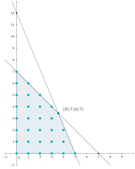
\[\begin{aligned} \min \quad & z = -80x_1 - 45x_2 \\ \text{s.t.:} \quad & x_1 + x_2 \leqslant 7 \\ & 12x_1 + 5x_2 \leqslant 60 \\ & x_1, x_2 \geqslant 0\\ & x_1, x_2 \in \mathbb{Z} \end{aligned}\]

Graphically, the set of integer solutions is shown in the following figure (light blue dots) alongside the continuous solution (dark blue diamond):

Root Node ($P_1$): Continuous Relaxation

We solve the problem by dropping the integrality condition on the variables ($x_1, x_2 \geqslant 0$ continuous):

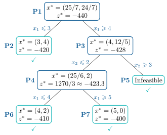
• Optimal solution: $x^* = \left(\frac{25}{7}, \frac{24}{7}\right) \approx (3.57, 3.43)$
• Objective function value: $z^* = -440$

Since neither $x_1$ nor $x_2$ are integer values, we must branch. We choose variable $x_1 = 3.57$ to split the problem into $x_1 \leqslant 3$ and $x_1 \geqslant 4$. In this way, we avoid the region $3 < x_1 < 4$ where no integer solution exists. The lower bound is set at $z_S = -440$.

Level 1: Branching on $x_1$

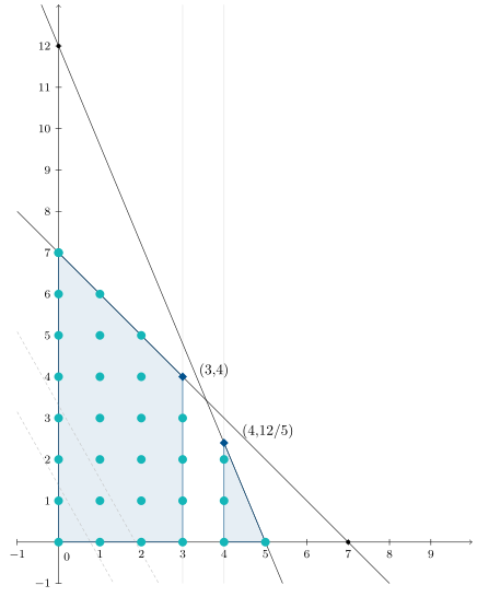
Once we decide to branch on variable $x_1$, the problems to solve graphically are $P_2$ (left side of the graph) and $P_3$ (right side of the graph):

• Subproblem $P_2$ ($x_1 \leqslant 3$)

  We add the constraint $x_1 \leqslant 3$ to the original problem and solve the new problem (using post-optimization techniques to save iterations):

  • Solution: $x^* = (3, 4)$
  • Objective value: $z^* = -420$

  The solution is integer, making it a feasible solution for the original problem.

  Being feasible and integer, we set our first known integer upper bound: $z_I = -420$. Therefore, it is no longer necessary to continue branching from $P_2$.

• Subproblem $P_3$ ($x_1 \geqslant 4$) We add the constraint $x_1 \geqslant 4$:

  • Solution: $x^* = \left(4, \frac{12}{5}\right) = (4, 2.4)$
  • Objective value: $z^* = -428$

  Since $z^* = -428 < z_I = -420$, this node can still yield a better solution than what we currently have. However, $x_2 = 2.4$ is not an integer, so we must branch $P_3$ with respect to $x_2$ into $x_2 \leqslant 2$ and $x_2 \geqslant 3$.

Level 2: Branching from $P_3$ on $x_2$

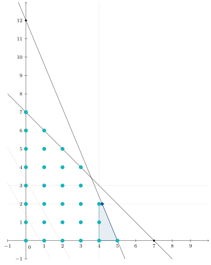
Branching $P_3$ on variable $x_2$, the problems to solve graphically are $P_4$ (bottom part of the graph) and $P_5$ (top part of the graph):

• Subproblem $P_4$ ($x_1 \geqslant 4, x_2 \leqslant 2$)

  • Solution: $x^* = \left(\frac{25}{6}, 2\right) \approx (4.17, 2)$
  • Objective value: $z^* = -\frac{1270}{3} \approx -423.33$

  Since $z^* = -423.33 < z_I = -420$ and variable $x_1 = 4.17$ is not an integer, we keep this node open to branch on it later.

• Subproblem $P_5$ ($x_1 \geqslant 4, x_2 \geqslant 3$)

  • Result: The system has no feasible region (Infeasible).

Level 3: Branching from $P_4$ on $x_1$

Branching $P_4$ on variable $x_1$, the problems to solve graphically are $P_6$ (left side of the graph) and $P_7$ (right side of the graph):

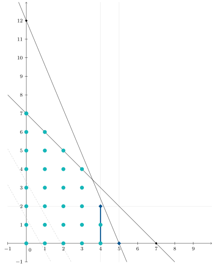
We branch node $P_4$ with respect to the fractional variable $x_1 \approx 4.17$ by evaluating $x_1 \leqslant 4$ and $x_1 \geqslant 5$.

• Subproblem $P_6$ ($x_1 \leqslant 4$, maintaining $x_1 \geqslant 4$ and $x_2 \leqslant 2 \implies x_1 = 4, x_2 \leqslant 2$)
  • Solution: $x^* = (4, 2)$ (Integer)
  • Objective value: $z^* = -410$
  • Analysis: Although integer, $z^* = -410 \geqslant z_I = -420$. This solution is worse than our known integer bound, so it is pruned.
• Subproblem $P_7$ ($x_1 \geqslant 5$, maintaining $x_2 \leqslant 2$)
  • Solution: $x^* = (5, 0)$ (Integer)
  • Objective value: $z^* = -400$
  • Analysis: Similarly, $z^* = -400 \geqslant z_I = -420$. It is pruned for failing to improve the bound.

Final Optimal Solution

There are no remaining nodes pending exploration. The best integer solution obtained throughout the process is from node $P_2$:

\[\mathbf{x}^* = (3,4) \quad \implies \quad z^* = -420\]

This entire procedure can be represented as a tree as follows:

Pruning Criteria and Exploration Strategies (Tuning)

The true power of Branch & Bound lies not only in partitioning the problem, but in knowing when to stop exploring a branch. If we had to explore the entire tree, the number of nodes would grow exponentially.

This is where algorithm tuning comes into play through pruning criteria and search strategies.

• Pruning Criteria (Closing Nodes)

  A node in the tree is considered complete (it is “pruned”) and is not branched further when one of the following three scenarios occurs:

  1. Pruning by Integrality: The relaxation of the subproblem produces a solution whose integer-restricted variables take on integer values. This solution becomes the new upper bound ($z_I$) if its value improves upon the best solution known so far.
  2. Pruning by Infeasibility: The subproblem generated by the new constraints has no feasible solution (as occurred at node $P_5$).
  3. Pruning by Bound (Dominance): The relaxed objective function value of the node ($z^$) is worse than or equal to the already known integer bound ($z^ \geqslant z_I$ in minimization). If the “relaxed” (ideal) version can no longer improve upon what we have already secured, its subsequent child solutions will not either.

• Tree Exploration Strategies

  The practical efficiency of the algorithm depends heavily on the order in which we select which node to explore next:

  • Depth-First Search (DFS): Explores a branch deeply until it quickly finds an integer solution. Its advantage is that it finds an upper bound $z_I$ early on, allowing bound-based pruning to start as soon as possible.
  • Breadth-First Search (BFS): Explores all nodes at the same level before descending deeper. It provides a global view of the bounds, though it consumes more memory.
  • Best-Bound Search: Selects the node with the most promising relaxed $z$-value. It is the preferred strategy for most modern solvers because it typically minimizes the total number of evaluated nodes.

Today, commercial and open-source solvers (such as Gurobi, CPLEX, or CBC) do not use pure Branch & Bound, but rather an evolved variant called Branch & Cut. This technique adds cutting planes (such as Gomory cuts) at each node to tighten the continuous relaxation before branching, solving industrial problems with millions of variables in seconds.

---

Branch & Bound demonstrates that you do not need to evaluate trillions of possible combinations in a discrete problem to find the optimal solution with complete mathematical certainty. Through continuous relaxation and the clever use of bounds, we can prune vast regions of the search space without ever exploring them.

---

Would you like to keep exploring the world of Operations Research? Discover more posts on the topic here.