Exploring linear optimization through graphical methods

Linear optimization is a powerful tool for making decisions, from scheduling production to allocating resources efficiently.

Even though real-world problems often involve many variables, the two-variable case is especially useful for learning. Graphical methods let you see the problem: what solutions are possible, where constraints lie, and why some solutions are better than others.

The graphical approach represents each constraint as a region on a plane and highlights the area where all constraints overlap. Suddenly, an abstract problem becomes a tangible geometric figure, making the idea of an optimal solution much easier to understand.

Setting up the problem

A linear optimization problem with two variables can be written as:

• Objective function: \(\max\; z = c_1 x_1 + c_2 x_2\) or \(\min\; z = c_1 x_1 + c_2 x_2\).

• Subject to linear constraints: \(a_{i1} x_1 + a_{i2} x_2 \leqslant b_i, \; \forall i = 1, \dots, m\).

• Decision variables: \(x_1\) and \(x_2\) (often assumed non-negative, \(\geqslant 0\)).

The goal is to find values of $x_1$ and $x_2$ that optimize $z$ while respecting all constraints.

Visualizing constraints and the feasible region

Intuitively, the feasible region contains all decisions that are allowed by the problem.

Each linear constraint defines a half-plane in $\mathbb{R}^2$. To draw a constraint:

1. Draw the line corresponding to the equality.
2. Determine which side satisfies the inequality.
3. Shade the feasible half-plane.

Non-negativity constraints keep the solution in the first quadrant.

The feasible region is simply the intersection of all these half-planes. Some key geometric facts are:

• The feasible region is convex.
• It can be bounded (a polygon) or unbounded.
• All feasible solutions lie within or on the boundary.

If no point satisfies all constraints, the problem is infeasible.

The objective function and optimality

The objective function can be pictured as a family of parallel lines:

\[z := c_1 x_1 + c_2 x_2 = k\]

Each $k$ gives a different line. Maximizing (or minimizing) the objective function consists of moving this line in the direction of improvement defined by the objective function coefficients while it still intersects the feasible region.

Graphically, the optimum is found where the line last touches the feasible region, usually at a vertex or extreme point. Sometimes, multiple optimal solutions lie along an edge (a segment in a bounded region or a ray in an unbounded region).

This leads to a key linear optimization result:

If an optimal solution exists, at least one occurs at a vertex of the feasible region.

Several situations may arise:

• Unique optimum: the objective function, at its optimum, touches the feasible region at a single vertex.
• Multiple optimal solutions:
  • Bounded region: the objective function, at its optimum, coincides with a segment on the boundary of the feasible region, i.e., a side of the polygon.
  • Unbounded region: the objective function, at its optimum, coincides with a ray on the boundary of the feasible region (the feasible region must be unbounded).
• Unbounded optimal solution: the objective function can improve indefinitely.
• Infeasible problem: there is no solution, i.e., the feasible region is empty.

In practice, feasible regions are usually bounded, because decision variables represent finite resources.

Illustrative Examples

We will explore examples showing all the scenarios dynamically with animations.

Unique Optimal Solution

Consider the following linear optimization problem:

\[\begin{aligned} \max\;\;& z = 6x_1 + 3x_2 \\ \text{s. t.:}\;\;& 2x_1 + 4x_2 \leqslant 8 \\ & -x_1 + 4x_2 \leqslant 4 \\ & x_1 - x_2 \leqslant 2 \\ & x_1, x_2 \geqslant 0 \end{aligned}\]

The animation shows the feasible region forming and the objective line moving until the optimum at a vertex:

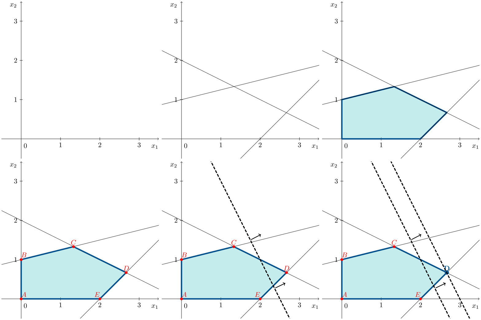
The optimal solution is at vertex $D=(8/3,2/3)^\intercal$, giving an objective function value, after substituting $x_1$ and $x_2$, of $z^* = 18$.

Multiple Optima in a Bounded Region

Consider:

\[\begin{aligned} \max\;\;& z = x_1 + x_2 \\ \text{s. t.:}\;\;& x_1 + x_2 \leqslant 8 \\ & -4x_1 + 4x_2 \leqslant 8 \\ & 2x_1 - x_2 \leqslant 6 \\ & x_1, x_2 \geqslant 0 \end{aligned}\]

The animation shows how, in this case, the objective function line coincides with an entire edge of the feasible region.

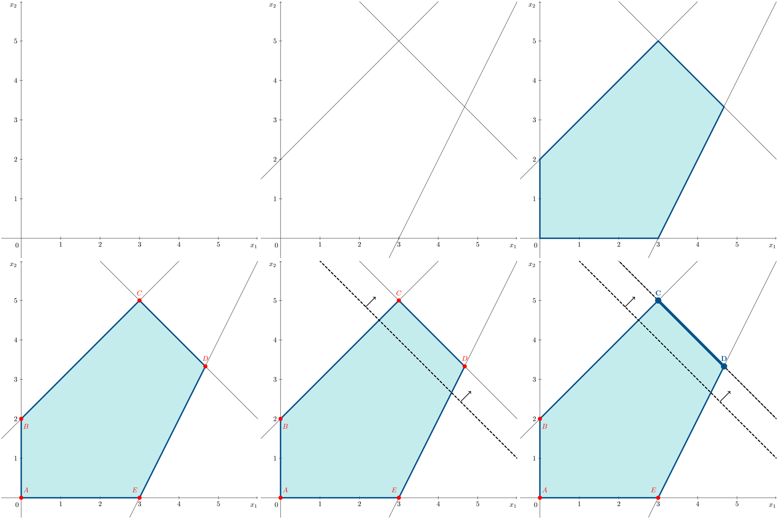
Vertices $C=(3,5)^\intercal$ and $D=(14/3,10/3)^\intercal$, as well as all points along the segment between them, are optimal. Therefore, the optimal solutions are the convex linear combination between points $C$ and $D$, given by:

\[\lambda \left(\begin{array}{c} 3 \\ 5\end{array}\right) + (1-\lambda) \left(\begin{array}{c} 14/3 \\ 10/3\end{array} \right), \quad \lambda \in [0,1]\]

with an objective function value $z^*=8$.

Multiple Optima in an Unbounded Region

Consider:

\[\begin{aligned} \min\;\;& z = x_1 \\ \text{s. t.:}\;\;& x_1 - x_2 \leqslant 2 \\ & 2x_1 + 2x_2 \geqslant 1 \\ & x_1, x_2 \geqslant 0 \end{aligned}\]

The animation shows how, in this case as well, the objective function line coincides with an entire edge of the feasible region.

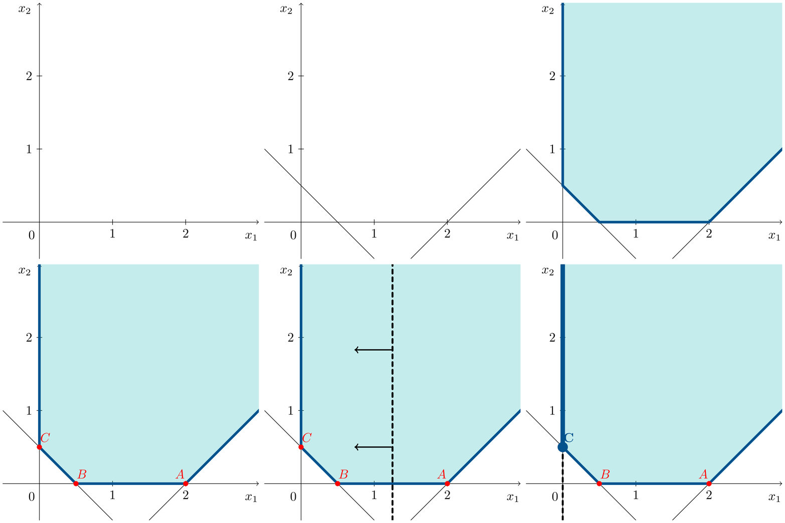
Vertex $C=(0,1/2)^\intercal$ is an optimal solution, together with the points on the ray starting from $C$ along the positive direction of the y-axis. The optimal solutions are given by:

\[\left(\begin{array}{c} 0 \\ 1/2\end{array}\right) + \mu \left(\begin{array}{c} 0 \\ 1 \end{array}\right), \quad \mu \geqslant 0\]

where the vertex and the vector defining the direction of the ray (or extreme direction) are taken into account. All these points yield the same objective function value, $z^*=0$.

Unbounded Optimal Solution

Consider:

\[\begin{aligned} \max\;\;& z = x_1 + 2x_2 \\ \text{s. t.:}\;\;& x_1 + 2x_2 \geqslant 2 \\ & -2x_1 + x_2 \leqslant 4 \\ & x_1, x_2 \geqslant 0 \end{aligned}\]

The animation shows how, in this case, the objective function line can move indefinitely, improving the solution without limit.

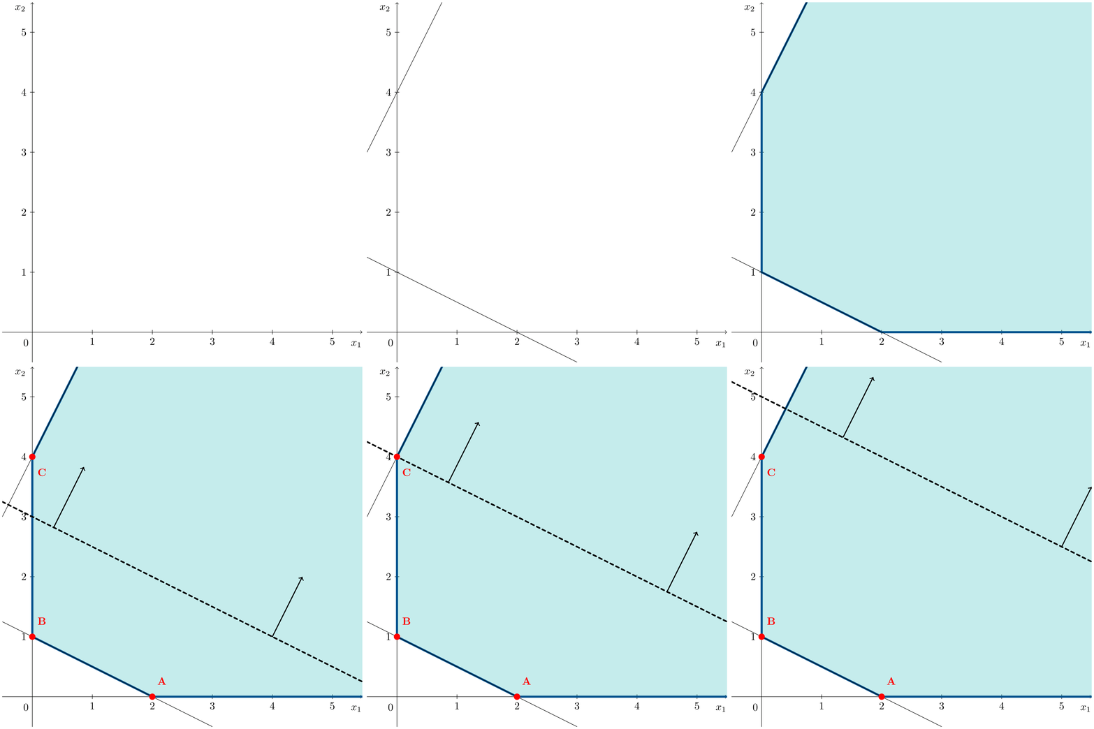
Following the direction of improvement of the objective function does not reach any vertex, allowing the objective function to increase as much as desired. In this case, the optimal objective value is $z^* = \infty$.

Infeasible Problem

Consider:

\[\begin{aligned} \min\;\;& z = x_1 + x_2 \\ \text{s. t.:}\;\;& 2x_1 + x_2 \leqslant 5 \\ & x_1 - x_2 \geqslant 4 \\ & x_1, x_2 \geqslant 0 \end{aligned}\]

The animation shows that, in this case, there is no intersection of the first quadrant with the two constraints.

The feasible region is empty, therefore, the problem is infeasible, and no solution exists that satisfies all constraints.

In all studied cases, the behavior of the solution depends exclusively on the geometry of the feasible region and the direction of the objective function. It is important to ensure that the objective function line moves in the correct direction according to the optimization criterion (maximization or minimization) and not to confuse unbounded region with unbounded optimal solution.

In two dimensions, solving a linear optimization problem consists of:

1. Constructing the feasible region.
2. Identifying its vertices and extreme directions.
3. Moving the objective line in the correct direction.
4. Analyzing the point or set of points where the optimum is reached (if it exists).

Limitations of the Graphical Method

The graphical approach is limited to problems with two or three decision variables. For higher-dimensional problems, algorithmic methods such as the Simplex Algorithm or Interior Point Methods are required.

Nevertheless, the geometric intuition acquired in two dimensions remains valid and serves as a foundation for understanding more advanced techniques. We can observe that:

• Convexity: The solution set of the problem is convex.
• Vertices or extreme points: They are the points potentially candidates to be the optimal solution.
• Extreme directions: Occur in problems with unbounded feasible regions, allowing to define the set of optimal solutions (in case of multiple optima) or the improvement direction when obtaining an unbounded optimal solution.
• Types of solution: Different conclusions can be drawn when solving the problem.

The graphical method provides a clear and intuitive way to understand linear optimization. Understanding this method is an important first step toward more general and powerful optimization tools. These geometric ideas are what allow reasoning to be generalized to methods like the Simplex, where it is no longer possible to draw the problem, but reasoning about vertices and extreme directions is still valid.