Uniform Search in Optimization: Measuring the Terrain Point by Point

Image by Jack Bain from Unsplash

The Uniform Search Method (also known as Exhaustive Grid Search or One-Dimensional Grid Search) is one of the most elementary and intuitive direct algorithms in numerical optimization. It is used to minimize or maximize a non-linear function of a single variable $f(x)$ over a closed and bounded interval $[a, b]$, without needing to calculate derivatives.

In the mid-20th century, with the birth of operations research and computational calculation in the 1950s and 1960s, the need arose to solve non-linear optimization problems where objective functions were complex, expensive to evaluate, or non-differentiable.

The formal study of one-dimensional search methods was systematized by Douglass J. Wilde in his famous book Optimum Seeking Methods (1964) (Wilde, 1964). Wilde classified non-linear search algorithms into two main categories:

1. Simultaneous Methods: All evaluation points are chosen in advance before performing any calculations.
2. Sequential Methods: Future evaluations depend on the results obtained in previous evaluations.

Uniform Search was established as the fundamental standard for simultaneous methods, serving as the conceptual foundation for the development of efficiency analysis in numerical optimization.

The Uniform Search Algorithm

The main objective of Uniform Search is to reduce the initial interval $[a, b]$ containing the global minimum of a continuous and unimodal function $f(x)$.

The algorithm operates based on the following steps:

1. Discretization: Given an integer \(n \geqslant 2\), we divide the interval $[a, b]$ into $n$ subintervals of equal length:

   \[\Delta x = \frac{b - a}{n}\]

2. Point generation: We generate $n + 1$ uniformly distributed points: \(x_i = a + i \cdot \Delta x \quad \text{for } i = 0, 1, 2, \dots, n\)

3. Evaluation: The objective function $f(x_i)$ is evaluated at each of the discretized points.

4. Localization of the minimum (maximum): The point $x_k$ that produces the lowest (highest) recorded value $f(x_k)$ is identified.

5. Subinterval of the minimum (maximum): By the unimodality property, the true minimum (maximum) $x^*$ is bounded within the subinterval formed by the neighbors of the found minimum (maximum) point:

   \[x^* \in [x_{k-1}, x_{k+1}]\]

   The length of the new interval is $2 \Delta x = \frac{2(b - a)}{n}$.

Pseudocode

Below is the structured algorithmic formulation:

\begin{algorithm}
\caption{One-Dimensional Uniform Search}
\begin{algorithmic}
\PROCEDURE{UniformSearch}{$$f, a, b, n$$}
    \STATE $$deltax = (b - a)/n$$
    \STATE $$xopt = a$$
    \STATE $$fopt = f(a)$$
    \STATE $$k = 0$$
    \FOR{$$i = 0$$ \TO $$n$$}
        \STATE $$xi = a + i * deltax$$
        \STATE $$val = f(xi)$$
        \IF{$$val < fopt$$}
            \STATE $$fopt = val$$
            \STATE $$xopt = xi$$
            \STATE $$k = i$$
        \ENDIF
    \ENDFOR
    \STATE $$liminf =$$\CALL{max}{$$a, a + (k - 1) * deltax$$}
    \STATE $$limsup =$$\CALL{min}{$$b, a + (k + 1) * deltax$$}
    \RETURN $$xopt, fopt, [liminf, limsup]$$
\ENDPROCEDURE
\end{algorithmic}
\end{algorithm}

Numerical Example

Let us consider the problem of minimizing the non-linear function:

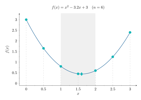
\[f(x) = x^2 - 3.2x + 3\]

over the interval $[a, b] = [0, 3]$ using $n = 6$ subintervals.

Analytically, by taking the derivative $f’(x) = 2x - 3.2 = 0$, we know that the minimum is located at $x^* = 1.6$ with $f(1.6) = 0.44$.

The step size is given by:

\[\Delta x = (3 - 0)/6 = 0.5\]

and the evaluation on the grid points:

$i$	$x_i = a + i \cdot \Delta x$	Evaluation $f(x_i) = x_i^2 - 3.2x_i + 3$
0	$0.0$	$(0)^2 - 3.2(0) + 3 = 3.00$
1	$0.5$	$(0.5)^2 - 3.2(0.5) + 3 = 1.65$
2	$1.0$	$(1.0)^2 - 3.2(1.0) + 3 = 0.80$
3	$1.5$	$(1.5)^2 - 3.2(1.5) + 3 = 0.45$
4	$2.0$	$(2.0)^2 - 3.2(2.0) + 3 = 0.60$
5	$2.5$	$(2.5)^2 - 3.2(2.5) + 3 = 1.25$
6	$3.0$	$(3.0)^2 - 3.2(3.0) + 3 = 2.40$

Looking at these results:

• The lowest function value achieved on the grid is $f(x) = 0.45$, reached at $x = 1.5$.
• Taking $x_k = 1.5$, the subinterval bounded by its adjacent points is: \(x^* \in [1.0, 2.0]\)
• Result: The initial search range of length $3.0$ has been reduced to a region of length $1.0$, guaranteeing that the optimum $x^* = 1.6$ lies inside.

The above procedure can be observed graphically in the following figure:

Technical Analysis and Practical Applications

For the final interval to have a width \(2\Delta x < \varepsilon\), a sufficiently large value of \(n\) must be chosen, given by:

\[\varepsilon > 2\Delta x = \frac{2(b-a)}{n}\]

and, therefore, one must choose:

\[n > \frac{2(b-a)}{\varepsilon}\]

Advantages, Limitations, and Practical Applications of the Algorithm

• Advantages:
  • Does not require derivatives: Works on non-differentiable or discontinuous functions.
  • Native parallelization: Being a simultaneous method, all $n$ evaluations are independent of each other and can be computed simultaneously on multiple cores or GPUs.
• Limitations:
  • The number of evaluations grows linearly with the desired precision, becoming inefficient if the computational cost of evaluating $f(x)$ is very high.

In current practice, Uniform Search is mainly used in hyperparameter optimization (Grid Search) in Machine Learning and as a preliminary exploration phase to bound regions of interest before applying local refinement methods.

Extension to the Multivariable Case

The principle of Uniform Search can be directly extended to the case of optimizing functions of multiple variables $f(x_1, x_2, \dots, x_d)$ over a bounded hyperrectangular domain $[a_1, b_1] \times [a_2, b_2] \times \dots \times [a_d, b_d]$.

In $d$ dimensions, instead of dividing a line segment, a grid or hypergrid is constructed in the parameter space. If we assign $n$ subintervals of equal size to each of the $d$ dimensions, we divide each axis $j$ with a step size:

\[\Delta x_j = \frac{b_j - a_j}{n}\]

The algorithm evaluates the function at all possible combinations of grid points and selects the coordinate tuple $(x_1, x_2, \dots, x_d)$ that minimizes $f$.

The Combinatorial Explosion

Although the conceptual extension is trivial, Uniform Search suffers drastically from what Richard Bellman called the curse of dimensionality.

The total number of numerical evaluations $N$ required to cover the space grows exponentially with the number of dimensions $d$:

\[N = (n + 1)^d\]

To illustrate this combinatorial growth:

• 1 variable ($d = 1$) with $n = 100$: requires $101$ evaluations (negligible).
• 2 variables ($d = 2$) with $n = 100$: requires $10,201$ evaluations (feasible).
• 3 variables ($d = 3$) with $n = 100$: requires $1,030,301$ evaluations (starts to become expensive).
• 5 variables ($d = 5$) with $n = 100$: requires $10,510,100,501$ evaluations (computationally unfeasible).

Each new variable multiplies the computational effort by a factor of $(n + 1)$, making it impossible to use fine grids when the search space has a moderate or high dimension.

For all these reasons, this method is not recommended for the multivariable case.

---

Uniform Search represents the cornerstone of uninformed optimization methods. Although its simplicity makes it inefficient for complex large-scale problems, its systematic sampling principle constitutes the conceptual foundation of modern techniques such as Grid Search in Machine Learning, proving that, before accelerating with gradients or heuristics, the first step is always knowing how to explore the terrain in an orderly and rigorous manner.

---

Want to keep exploring the world of Operations Research? Discover more posts on the topic here.